
Modelling Your Queues
Let’s model a distributed platform as a series of queues.
Here I’ll be using Simmer to model the performance of a real-world analytics platform. Simmer is
a process-oriented and trajectory-based Discrete-Event Simulation (DES) package for R
It allows us to model a process as a “trajectory” an item takes through various stages or “resources” in Simmer parlance.
A Simple Platform
Let’s imagine we have a very simple system that receives a measurement via REST API, performs some analysis, and writes that analysis to the database. We’ll need the simmer library for this:
library(simmer)
## Warning: package 'simmer' was built under R version 3.6.2
library(parallel)
library(simmer.plot)
We now create a simple platform “environment”:
set.seed(42)
simplePlatform <- simmer("SimplePlatform")
We now set up the process steps our measurement will follow - the trajectory. Our trajectory for a measurement is to be received by an “api”, then to be analysed by an “analyser” and finally written to the database by a “database” resource:
measurement <- trajectory("measurements") %>%
  seize("api") %>%
  timeout(function() rnorm(1, 15)) %>%
  release("api") %>%
  seize("analyser") %>%
  timeout(function() rnorm(1, 20)) %>%
  release("analyser") %>%
  seize("database") %>%
  timeout(function() rnorm(1, 5)) %>%
  release("database")
Note that each process step is declared in 3 parts:
- seize() which states what resource will be used for the step
- timeout() which is a variable delay - here supplied by an rnorm() distribution
- release() which states what resource is released at the end of the step
Note that the time units are independent of any particular time scale - for one system it could be microseconds, for another it could be minutes, hours, days etc.
Now we can setup the simulation environment resources - we’ll have one api, one analyser and one database:
simplePlatform %>%
  add_resource("api", 1) %>%
  add_resource("analyser", 1) %>%
  add_resource("database", 1) %>%
  add_generator("measurement", measurement, function() rnorm(1, 10, 2))
## simmer environment: SimplePlatform | now: 0 | next: 0
## { Monitor: in memory }
## { Resource: api | monitored: TRUE | server status: 0(1) | queue status: 0(Inf) }
## { Resource: analyser | monitored: TRUE | server status: 0(1) | queue status: 0(Inf) }
## { Resource: database | monitored: TRUE | server status: 0(1) | queue status: 0(Inf) }
## { Source: measurement | monitored: 1 | n_generated: 0 }
Above we see a view of the current configuration.
Now we can run the simulation for 80 time units:
simplePlatform %>%
  run(80)
## simmer environment: SimplePlatform | now: 80 | next: 81.2899274063862
## { Monitor: in memory }
## { Resource: api | monitored: TRUE | server status: 1(1) | queue status: 2(Inf) }
## { Resource: analyser | monitored: TRUE | server status: 1(1) | queue status: 1(Inf) }
## { Resource: database | monitored: TRUE | server status: 0(1) | queue status: 0(Inf) }
## { Source: measurement | monitored: 1 | n_generated: 8 }
We can plot the usage for the single run:
resources <- get_mon_resources(simplePlatform)
plot(resources, metric = "usage", c("api", "analyser", "database"))
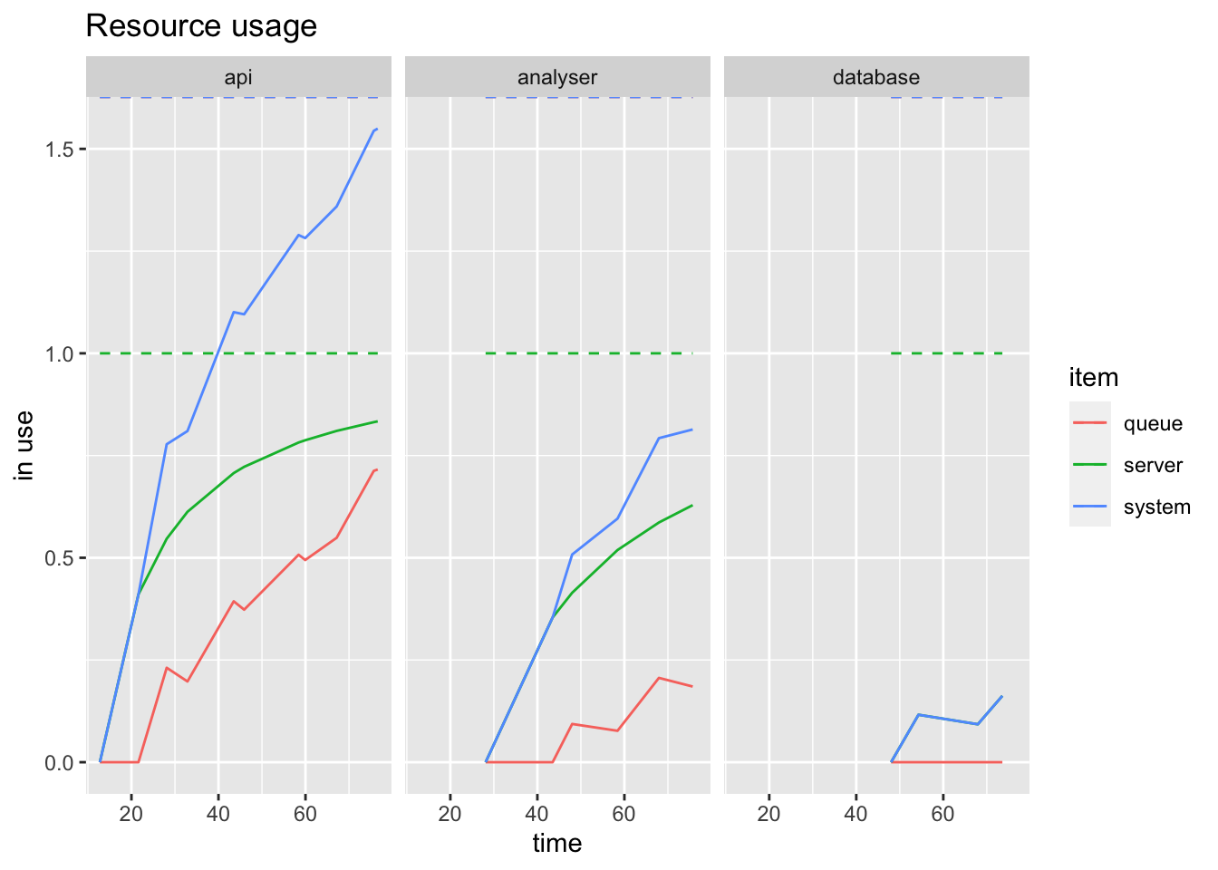
Here the server line shows how the resource is used, whereas the queue line shows the queues filling up. The system line is the sum of both.
Now let’s look at a more complicated example.
A Real World(ish) Example
Let’s try again with a subset of a real analytics platform. It receives measurements as before, but they are not always in the right format - these measurements are pre-processed into a standard format; the processed data is then distributed to several analysers which perform different types of analysis independently (i.e. in parallel); finally the results of all of these are written to the same database. Let’s have two different analysis steps.
There is one further complication: each of the steps needs to use the database. We will model this by seizing and releasing the “database” resource as part of each step.
Here is the platform:
realPlatform <- simmer("RealPlatform")
Here is the trajectory for the raw messages:
raw_data <- trajectory("raw data pre-processing") %>%
  seize("api") %>%
  seize("database") %>%
  timeout(function() rnorm(1, 15)) %>%
  release("database") %>%
  release("api") %>%
  seize("preprocessor") %>%
  timeout(function() rnorm(1, 20)) %>%
  release("preprocessor")
Here is the trajectory for the first analyzer:
analysis1 <- trajectory("analysis type 1") %>%
  seize("analyzer1") %>%
  seize("database") %>%
  timeout(function() rnorm(1, 15)) %>%
  release("database") %>%
  release("analyzer1") %>%
  seize("database") %>%
  timeout(function() rnorm(1, 20)) %>%
  release("database")
Here is the trajectory for the second analyzer:
analysis2 <- trajectory("analysis type 2") %>%
  seize("analyzer2") %>%
  seize("database") %>%
  timeout(function() rnorm(1, 15)) %>%
  release("database") %>%
  release("analyzer2") %>%
  seize("database") %>%
  timeout(function() rnorm(1, 20)) %>%
  release("database")
We can now build the whole trajectory for the system. Here we use the clone() function to create a paralle fork between the two analyzers:
whole_trajectory <- trajectory() %>%
  join(raw_data) %>%
  clone(
    n=2,
    join(analysis1),
    join(analysis2)
  )
Now let’s setup the resources:
realPlatform %>%
  add_resource("api", 1) %>%
  add_resource("preprocessor", 2) %>%
  add_resource("analyzer1", 2) %>%
  add_resource("analyzer2", 2) %>%
  add_resource("database", 1) %>%
  add_generator("whole_trajectory", whole_trajectory, function() rnorm(1, 10, 2))
## simmer environment: RealPlatform | now: 0 | next: 0
## { Monitor: in memory }
## { Resource: api | monitored: TRUE | server status: 0(1) | queue status: 0(Inf) }
## { Resource: preprocessor | monitored: TRUE | server status: 0(2) | queue status: 0(Inf) }
## { Resource: analyzer1 | monitored: TRUE | server status: 0(2) | queue status: 0(Inf) }
## { Resource: analyzer2 | monitored: TRUE | server status: 0(2) | queue status: 0(Inf) }
## { Resource: database | monitored: TRUE | server status: 0(1) | queue status: 0(Inf) }
## { Source: whole_trajectory | monitored: 1 | n_generated: 0 }
Let’s run this simulation as before and plot the usage:
realPlatform %>%
  run(80)
## simmer environment: RealPlatform | now: 80 | next: 81.164941511184
## { Monitor: in memory }
## { Resource: api | monitored: TRUE | server status: 1(1) | queue status: 4(Inf) }
## { Resource: preprocessor | monitored: TRUE | server status: 0(2) | queue status: 0(Inf) }
## { Resource: analyzer1 | monitored: TRUE | server status: 2(2) | queue status: 0(Inf) }
## { Resource: analyzer2 | monitored: TRUE | server status: 2(2) | queue status: 1(Inf) }
## { Resource: database | monitored: TRUE | server status: 1(1) | queue status: 5(Inf) }
## { Source: whole_trajectory | monitored: 1 | n_generated: 9 }
resources <- get_mon_resources(realPlatform)
plot(resources, metric = "usage", c("api", "preprocessor", "analyzer1", "analyzer2", "database"))
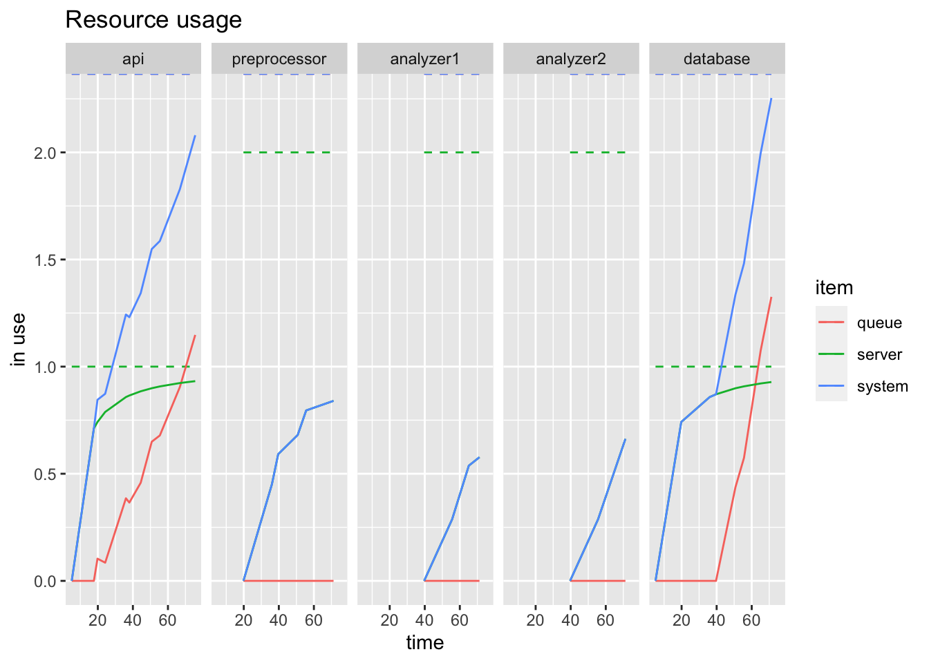
It’s quite easy to see how the single database quickly reaches capacity while the intermediate steps don’t. You probably didn’t need a process model to guess that this would be the case, but with this model you can now plug in real numbers and hypothetical architectural changes to see what would happen.
We can go further with simmer - adding rejections, more complex behaviour at each step and so forth. Check out the simmer examples for more ideas.
