
Estimating R In The UK
Note this post needs revision as the method of calculating R0, especially after the peak, is incorrect - see here for details
I have written previously about the R0 package and how it can be used to estimate R, and I have used this to build a Shiny app to re-calculate R on demand with the latest data. In the app, I make a rather wildly inaccurate, or rather, unstable prediction about when the peak or plateau will end by using the slope of R. This instability magnifies the underlying uncertainty in estimated R over time, which in turn depends on the accuracy of the data and the R0 model.
What is the consensus value for R across the UK as I write this (12th May 2020)? According to this BBC article, R is currently in the range 0.75 to 1 (according to Imperial College London?). What does the R0 package with the “time-dependent” model say:
library(tidyverse)
library(lubridate)
library(R0)
confirmed <- read.csv(url("https://raw.githubusercontent.com/CSSEGISandData/2019-nCoV/master/csse_covid_19_data/csse_covid_19_time_series/time_series_covid19_confirmed_global.csv"))
confirmed <- subset(confirmed, select = -c(Lat, Long))
ukConfirmed <- confirmed %>%
filter(Country.Region == "United Kingdom")
sums <- colSums(ukConfirmed[,-match(c("Province.State", "Country.Region"), names(ukConfirmed))], na.rm=TRUE)
sumsByDateCode <- as.data.frame(t(t(sums)))
colnames(sumsByDateCode) <- c("count")
sumsByDateCode$datecode <- rownames(sumsByDateCode)
dailyCounts <-mutate(sumsByDateCode, date = mdy(substring(datecode, 2)))
dailyCounts$day <- seq.int(nrow(dailyCounts))
dailyCounts <- dailyCounts %>%
filter(count > 0)We’ll continue to use a generation time distribution with a mean of 5 days, standard deviation 1.9:
meanGenerationTime <- generation.time("gamma", c(5, 1.9))Let’s estimate R:
est <- estimate.R(dailyCounts$count, methods=c("TD"), GT=meanGenerationTime)estimatedR <- est$estimates$TD$R[1:length(est$estimates$TD$R)-1]
estimateRByDay <- as.data.frame(estimatedR) %>%
rename(R = estimatedR) %>%
mutate(day = row_number())
plot(estimateRByDay$day, estimateRByDay$R, xlab="days", ylab="R", type="l", main="Effective R")
abline(h=1, col="gray60")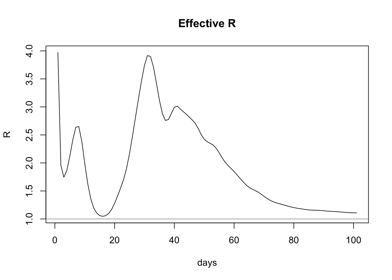
This model predicts that the latest value of R is 1.1087439, which is above the aforementioned range. Critically, it’s above 1.
So, can we quantify the errors in our estimate? For starters, the R0 package estimation produces a 95% confidence interval, which we can plot. Note that the confidence interval variable contains data for one day in the future, so we’ll slice it off before plotting:
confInt <- est$estimates$TD$conf.int %>%
  mutate(day = row_number()) %>%
  slice(-n())

plot(estimateRByDay$day, estimateRByDay$R, xlab="days", ylab="R", type="l", main="Effective R")
abline(h=1, col="gray60")
lines(confInt$day, confInt$upper, col="orange")
lines(confInt$day, confInt$lower, col="orange")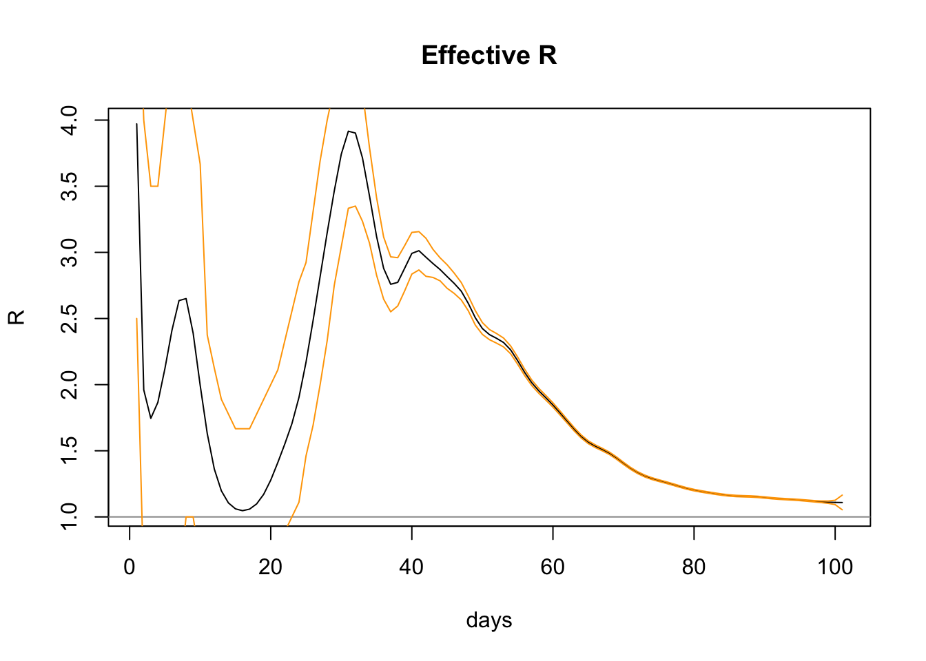
The graph shows increasing confidence (ie narrower bands) as more data comes in and the slope settles down. The upper and lower confidence levels (shown above in orange) have a range on the last day of 1.0540665 to 1.1647471, so the R0 package is pretty confident with the figure 1.1087439.
So, setting aside R for a moment, what does the predicted case data look like, compared to actual case data? Note the predicted case data day 1 starts from the first case, which happens on day 10, so we need to offset our predictions to match this:
predictedCases <- as.data.frame(est$estimates$TD$pred) %>%
  rename(prediction = "est$estimates$TD$pred") %>%
  mutate(day = row_number() + dailyCounts$day[1]) %>%
  slice(-n())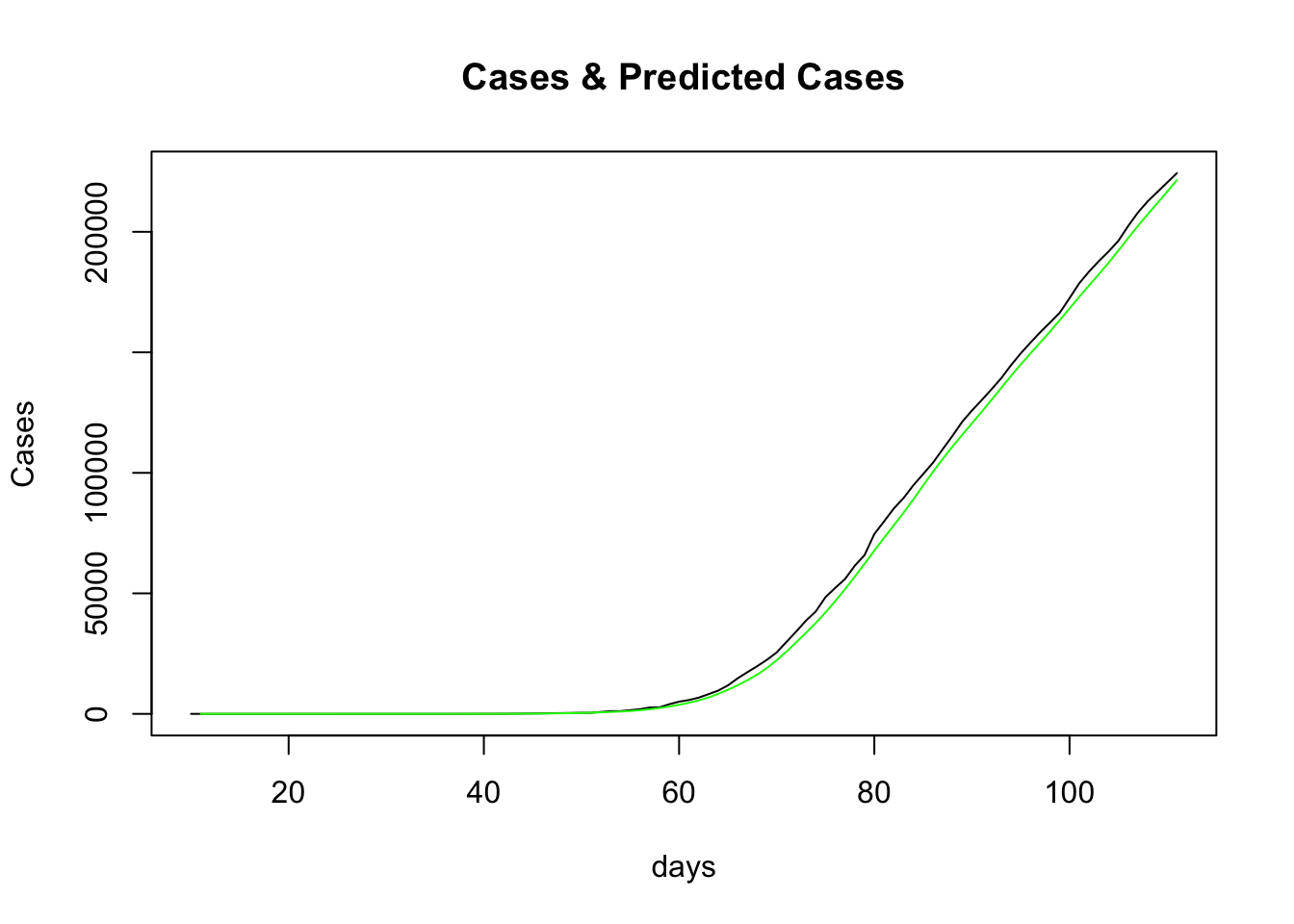
The actual cases are in black and the predictions in green. This doesn’t look like a bad fit either. Indeed it was seen previously that the “time-dependent” method produced a better fit than all the other options that the R0 package supplies.
We can see what the other methods the latest estimate of R to be easily enough:
allMethodsEstimate <- estimate.R(dailyCounts$count, methods=c("TD", "EG", "ML", "SB"), GT=meanGenerationTime)

lastDay <- allMethodsEstimate$end -1

timeDependentR <- allMethodsEstimate$estimates$TD$R[lastDay]
exponentialGrowthR <- allMethodsEstimate$estimates$EG$R
maximumLikelihoodR <- allMethodsEstimate$estimates$ML$R
sequentialBayesianR <- allMethodsEstimate$estimates$SB$R[lastDay]

variousRs <- data.frame(method=factor(), R=numeric())

variousRs <- variousRs %>%
  add_row(method="Time-Dependent", R=timeDependentR) %>%
  add_row(method="Exponential Growth", R=exponentialGrowthR) %>%
  add_row(method="Maximum Likelihood", R=maximumLikelihoodR) %>%
  add_row(method="Sequential Bayesian", R=sequentialBayesianR)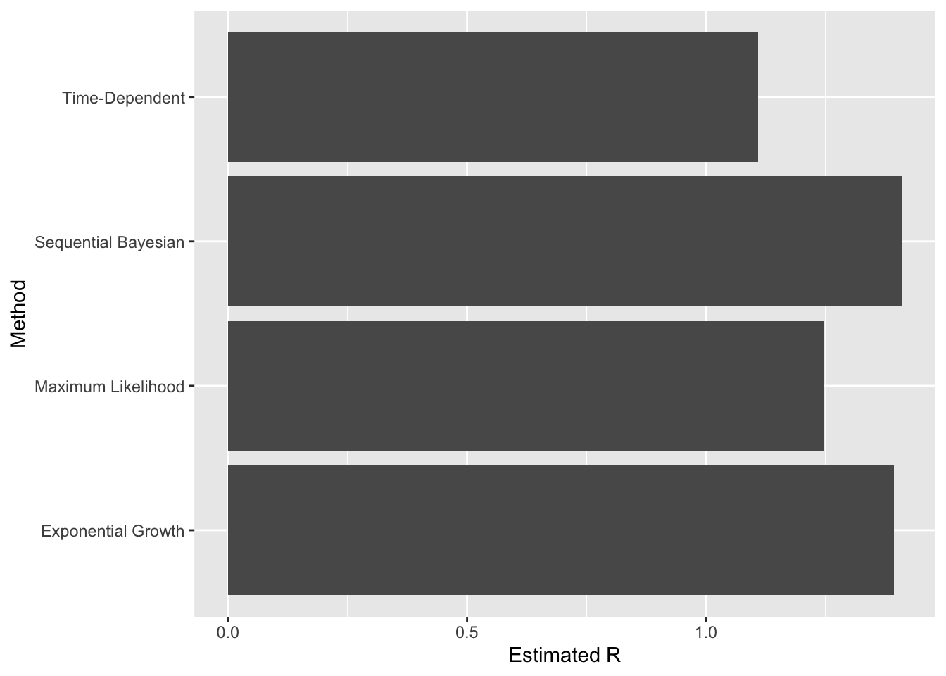
The “Time-Dependent” method still aligns more closely with the published range of 0.75-1.0.
Is the generation time a factor? I used the distribution of 5 days with a standard deviation of 1.9, as per this paper. What effect does varying this have?
This CDC article reports a generation time with a distribution with a mean of 3.96 days and a standard deviation of 4.75 days. Using the “time-dependent” method, what is the most recent estimated R value?
est2 <- estimate.R(dailyCounts$count, methods=c("TD"), GT=generation.time("gamma", c(3.96, 4.75)))

estimatedR2 <- est2$estimates$TD$R[est2$end-1]
With this generation time, the estimated most recent R is 1.1079562. This isn’t significantly different.
Very roughly speaking, the higher the generation time, the larger R is estimated to be. Compare the estimates for a generation time mean of 20 days versus 1 day:
estHigh <- estimate.R(dailyCounts$count, methods=c("TD"), GT=generation.time("gamma", c(20, 1)))
estimatedRHigh <- estHigh$estimates$TD$R[estHigh$end-1]

estLow <- estimate.R(dailyCounts$count, methods=c("TD"), GT=generation.time("gamma", c(1, 1)))
estimatedRLow <- estLow$estimates$TD$R[estLow$end-1]
The 20 -day estimate is 1.7229135 whereas the 1-day estimate is 1.0286179. While these differences are very critical when considering the R=1 boundary, it doesn’t look like different generation time estimates would get us close to the 0.75-1.0 range with the given case data.
I haven’t managed to find any specific details about how the published R values are produced. I think I will have to spend more time digging through the Imperial College London COVID-19 scientific resources to find out.
